Introduction

In the financial crisis, equities markets lose their diversification properties because they become highly correlated. Further, because of low and negative relationships of commodities market with equity, investors diversify their portfolio to commodities. However, to get the benefits of diversification, the risk-return trade-off should hold and it should be steady. We study the stability and trade-off of risk and return for the two most popular diversifiable commodity assets such as gold and copper, so that portfolio optimisation could be achieved by including both the assets into the portfolio.

Theoretically, Risk and Return trade-off properties are inconclusive Rossi and Timmermann (2010). Also, empirical findings are inconclusive.1 The conflicting results could be attributed to the omitted variable bias. Models suffer from omitted variable bias as it has been seen that the trade-off is affected by not only local and regional factors but also by global factors, Aslanidis et al. (2016), investment opportunities, Scruggs (1998) and Guo and Whitelaw (2006), consumption-wealth ratio, Lettau and Ludvigson (2001), lagged mean and volatility, Lettau and Ludvigson (2010), to mention a few.

Further, because of non-linearity and existence of jumps in time series, linear models are suffering from specification error in risk-return trade-off studies. Again non-linear studies on risk-return trade-off using a regime switch or time-varying framework suffer from restrictive assumptions about the data-generating process (i.e., no of regimes) (Thies & Molnar, 2018).

We have applied Bayesian change point detection, see Ruggieri and Antonellis (2016), allied to a novel variability regime selection to investigate whether commodity2 returns are risk-adjusted through which we are taking care of omitted variable bias, the non-linearity without any restrictive assumptions about data generating process and the asymmetric dynamics as well by constructing regimes with similar risk-return trade-off. We have taken gold from bullion and copper from base metal segment because it has been seen during crisis that base metal and bullion commodities share a less or negative relationship with other asset classes.

In the first stage, segments are identified along with their corresponding posterior probability in the distribution of gold and copper return through break-points using Bayesian break-point analysis. The identified breakpoints and segments explain the stability of the risk-return parameters across time. In the second stage, we have investigated whether the risk-return trade-off holds, a notably positive trade-off which is the reflection of the fact that the investors are risk averse who demand more returns for bearing additional risk. We have merged the segments with similar statistical properties identified in the first stage into regimes which reveals the sign and size of the risk-return trade-off. Each regime so established will describe a particular level of volatility with its corresponding size and sign of the return. To the best of our knowledge, our study is the first of its kind to apply Bayesian change point analysis in commodities market from portfolio management prospective.

We find that risk-return trade-off dynamics across commodities markets and across volatility regimes are different. Gold emerges as the safe heaven investing commodity for portfolio diversification during a high volatility regime. However, in a low volatility regime, both copper and gold lose their diversification properties because the risk-return trade-off becomes negative.

The remaining part of the paper is organised as follows. Section 2 explains the data and its descriptive statistics. Section 3 discusses the methodology used in the study. Section 4 presents the empirical analysis and section 5 concludes the paper.

Data

Daily gold (from 10/11/2003 through 30/11/2017) and copper (from 04/06/2004 through 30/11/2017) price data starting from the date of their respective trading have been collected from www.mcxindia.com, the official website Multi Commodity Exchange. The descriptive statistics of the return series measured as log (Pt/Pt-1) are presented in Table 1.

The unconditional maximum return, although average return looks same and standard deviation indicates copper as a high-return and high-risk commodity in comparison to gold. But as BDS test results show that both are non-linear, the unconditional risk-return trade-off may not hold across time. Both the return series are stationary as per the KPSS, PP, and Zivot–Andrew breakpoint unit root test. High Kurtosis and negative skewness further characterise both series as leptokurtic and slightly asymmetric.

Methodology

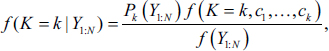
Based on the Ruggieri and Antonellis (2016) Bayesian multiple change-point detection allied with multiple-sample variance tests, a time series Y_t, N ×1 is subdivided into regimes of same variance based on X_t, N ×m, that is, the information. Based on the assumption that a structural break occurs at a given date where f(ck)>η, for some η∈(0,1), the posterior probability, f(ck)  is calculated at a specific location for the change point. After the identification of breakpoints, a statistical test is applied to find out whether the variances of each subset of the time series are indistinguishable. Therefore, statistically, each regime is defined as the subsets of equal variance.

 

Table 1. Descriptive Statistics of Daily Gold and Copper Return.

Notes: *Significance at 1% level.

Std Dev. is the standard deviation.

 

The Bayesian approach of Ruggieri and Antonellis (2016) in detecting structural change points is an extension of Ruggieri (2012). The main difference between those methods is that the first can handle new observations without processing the entire series once more. This feature is desired since the Ruggieri (2012) method results in exponential time consuming as the number of observations increases.

Following are the three steps proposed by Ruggieri (2012) in the algorithm for the Bayesian approach to detect change points.

1. Calculation of fYi:jX, that is, the probability density for all the possible substrings of the data, Yi:j, with 1≤i.
2. Let PkY1:jbe the density of the data [Y1…Yj] with k change points. For k>0, define
3. Where P0(Y1:v)=f(Y1:v)  is calculated by Step 1.
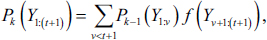
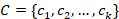4. Assuming  change points, with location designed by C={c1,c2,…,ck}, with a prior `uniform change points location distribution on, that is, f(c1,…,ck|K=k)=1/Nk, where the possible number of solutions containing k change points is Nk. Then, we have,

            

            

                   

             when k=1, P0(Y1:v)=f(Y1:v) is given by Step 1.

            The previous algorithm is altered in Ruggieri and Antonellis (2016) where the values of the first and second steps are stored in two matrices which is used to update the dynamic programming recursion. Thus, we have for a  new observation, 

          
            

             for k=1 to kmax. The posterior distribution on the number of change points is now given by,

           

            and for a detected change point, the exact posterior distribution of the location is given by,

               

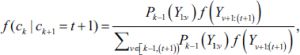
where ck is the location of the th change point and ck+1=t+1  be the newest observation.

Given the posterior distribution of the set of location of change points, the regimes of statistically equal variance is defined using the algorithm as follows:

1. According to the probability of structural break, the initial regime is defined for a threshold probability η, if the change point probability, f(ck), is below the threshold value η, the observation is said to be from the previous regime.
2. Initial regimes having same variance is clustered to update the regimes set R by following the procedures mentioned below:

• For a given probability of rejection α, statistical test is conducted whether the variability of Regime i  is identical to the Regime j, j>i.
• If the null hypothesis of equal variance is not rejected, the new Regime i is given by Regime i* = Regime i ∪ Regime j and R={…, Regime i*,…} 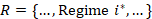- Regime j.

 Section 4 presents results for Bartlett’s equal variances test using η=0.10, α=0.05. Additionally, the gold and copper returns series were standardised with mean and standard deviation zero and one respectively. As far as dependent variable is concerned, date is converted from string to numerical.

Empirical Analysis

The nature of risk-return trade-off is different for both gold and copper. The sign (return) and size (volatility) dynamics are also different. The relationship between return and risk is mixed. The risk-return trade-off is not stable for both commodities over the period of the study.

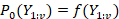
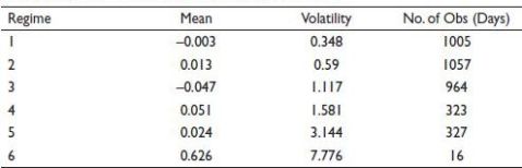
Jumps in return and volatility clustering in the upper part of Figure 1(a) and Figure 2(a) and its further segmentation based on posterior volatility in the lower part of the figure throws some interesting fact about the change point and corresponding risk-return trade-off in both copper and gold, respectively. The certainty in the timing of the change point can be observed from the posterior probability graph, see Figure 1(b) and Figure 2(b) where the height of these spikes is an indicator of the probability of selecting a change point in time. One thing that stands out is the strong variation in posterior mean and volatility with different lengths of the identified segment. It is an indication of the fact that the transition between segments (i.e., from one point in time to another) is abrupt and continuous lasting after that for a specified period. Strong variation in posterior mean and volatility across segments in both gold and copper is an indication of the fact that the risk-return trade-off is not stable. For example, copper returns sudden change from one regime to another is observed in January 2008 and April 2008 and thenceforth lasts for several months from April 2008 to March 2011. However, gold returns changing regimes do not occur at the same moment as reported for copper returns series, thus showing a different risk-return trade-off structure. An abrupt change point was observed in August 2005 subsequently lasted for a very short period. However, the regime followed by October 2005 and December 2008 lasted for almost two years. To further understand the time series dynamics, we combine the segments revealing same statistical properties into regimes that are presented in Table 2 and Table 3 for copper and gold returns, respectively. We observe six regimes exhibiting interesting risk-return dynamics, which has implications for portfolio construction. The risk-return trade-off is different for gold and copper returns regarding both sign and size. In case of gold, the positive risk-return trade-off holds in higher volatility regime starting from regime four with a mean return of 0.051 and volatility of 1.581 to regime six with a mean return of 0.626 and volatility of 7.776, despite holding only for a very short period. However, for copper in the higher volatility regime, the risk-return dynamics does not hold where the relationship is negative. So that means the portfolio managers should include gold in their portfolio and disinvest from copper in higher volatility regime. However, in low volatility regime, that is, from regime one through three both copper and gold lose the diversification properties as positive risk-return trade-off does not hold. That means in highly uncertain economic and financial environment only gold can be included in the portfolio to get the diversification benefit.

Figure 1. Part (a) Upper Part Shows the Return and Volatility Clustering of Copper with Posterior Mean and Posterior 95%-interval and Lower Part Shows the Regimes Based on Clustering of Independent Segments by their Posterior Volatility. Part (b) Presents the Posterior Probability Associated with Change Points Copper Return. The Height of the Spike Indicates the Probability of Selecting a Change Point at a Specific Point in Time.

 

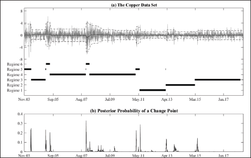
Figure 2. Part (a) Upper Part Shows the Return and Volatility Clustering of Gold with Posterior Mean and Posterior 95%-interval and Lower Part Shows the Regimes Based on Clustering of Independent Segments by their Posterior Volatility. Part (b) Presents the Posterior Probability Associated with Change Points Gold Return. The Height of the Spike Indicates the Probability of Selecting a Change Point at a Specific Point in Time.

 

Table 2. Regime-wise Mean and Volatility of Copper Return.

 

 

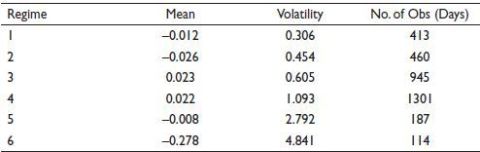
Table 3. Regime-wise Mean and Volatility of Gold Return.

 

 

Conclusion

The stability and trade-off of risk-return are fundamental to portfolio investing and also at the time of crisis commodities are considered as safe heaven investing. Further, both theoretically and empirically the risk-return trade-off relationship is inconclusive. However, since both theoretically and empirically the risk-return trade-off relationship is inconclusive, the portfolio manager should know the point of change, thereafter duration of the change period with certainty. We have applied a Bayesian change point methodology and proposed a novel variability regime selection to two most popular commodities copper and gold which are typically considered as portfolio diversification because of their low or negative relationship with other financial assets. We find that in higher volatility regime only gold can be considered as a diversifiable commodity because positive risk-return trade-off holds. However, in low volatility regime both of the commodities lose their diversification properties as the risk-return relation becomes negative. Thus, the portfolio manager could disinvest in commodity assets like gold and copper in low volatility regime, but she could add gold into the portfolio to reap the benefits of diversification.

Declaration of Conflicting Interests

The authors declared no potential conflicts of interest with respect to the research, authorship and/or publication of this article.

Funding

The authors received no financial support for the research, authorship and/or publication of this article.

Notes

Significantly negative conditional relationship Campbell (1987), Nelson (1991) and Brandt and Kang (2004), Positive and significant Ghysels et al. (2005), Ludvigson and Ng (2007). Positive and mostly insignificant French et al. (1987), Baillie and DeGennaro (1990), Campbell and Hentschel (1992), both positive and negative which depend on methodology being used Harvey (1989) and Glosten et al. (1993).

The studies so far are mostly focussed on the equity market and that to US, European and Pacific Basin stock markets.