
IMIB Journal of Innovation and Management

 Search

Rohit Vishal Kumar1
1 International Management Institute, Bhubaneswar, Odisha, India

Creative Commons Non Commercial CC BY-NC: This article is distributed under the terms of the Creative Commons Attribution-NonCommercial 4.0 License (http://www.creativecommons.org/licenses/by-nc/4.0/) which permits non-Commercial use, reproduction and distribution of the work without further permission provided the original work is attributed.
The most widely used metric for assessing a scale’s reliability is Cronbach’s alpha. Since its introduction in 1951 by Lee Cronbach, it has evolved into the accepted benchmark for scale reliability. A quick search for ‘Cronbach’s alpha’ in Google Scholar yields more than 8 hundred thousand results. By any measure, this is enormous, and the usage of alpha appears to be present in practically every domain of academics. The fact that alpha has been so successful is surprising, as researchers have consistently criticised and have pointed out a plethora of problems with it. For instance, is that Cronbach never suggested alpha as a reliability metric—rather he proposed alpha as an alternative measure for equivalency in a test-retest context. Another issue Cronbach never suggested the lower bound of 0.70 as a benchmark of reliability. However, the lower bound of 0.70 has become the holy grail of scale reliability. Alpha continues to lead all measures of scale reliability despite its numerous issues. This article examines the history of alpha, its derivations based on classical test theory, and its limitations. It then suggests three alternative measures, along with software procedures to calculate them: alpha with confidence interval, omega and greatest lower bound. The purpose of this article is to enable researchers to have a better idea about the limitations of Cronbach’s alpha, and to make them aware of other measures of reliability which are available. It is hoped that this article will help researchers report better and more accurate reliability measures in their research works alongside the alpha.
Reliability, scale development, Cronbach’s alpha, McDonald’s omega, greatest lower bound
Introduction
Measurement is an integral part of the modern world, but its origins can be traced back to the barter system. Before a farmer could agree to barter his produce, he needed to establish a common ground on which the exchange could take place. Fortunately, in the natural sciences, measurement systems evolved at a rapid pace and were accepted worldwide. However, developing measurement systems in the social sciences proved to be more difficult as social scientists were forced to measure abstract concepts. For example, measuring ‘happiness’ is not as easy as asking how happy you are? Social, economic, legal and other factors determine the meaning of happiness. Despite these issues, it became necessary to measure these abstract concepts, to provide accurate information for decision-making in various fields. This requirement for measuring items that were not directly observable led to a huge interest in the development and validation of such scales in psychology and related fields.
For some reason, Cronbach’s alpha has become the standard on which the reliability of such measurements is judged. However, to quote the famous author, ‘The numerous citations to my article by no means indicate that the person who cited it had read it’ (Cronbach & Shavelson, 2004). Such a strong criticism from the author has not dented the image of alpha, and it continues to be cited with aplomb by researchers worldwide.
This article examines the evolution of Cronbach’s alpha, the limitations associated with its use, and a few alternative approaches. In part two, we provide a concise overview of the reliability measures before alpha. Part three covers the classical test theory (CTT), whereas part four focuses on the derivation of alpha. Part five covers the concerns related to alpha, while part six explores three alternatives to alpha: alpha with confidence intervals (CIs), McDonald’s omega and the greatest lower bound (GLB). Part seven employs a readily accessible data set to illustrate the computation of different options. This work aims to enhance scholars’ comprehension of the issues involved with Cronbach’s alpha, while also stimulating consideration of alternative metrics.
Reliability Measures Before Alpha
Reliability has been one of the main concerns of researchers for a long time; however, reliability is not easily determined in the real world. To accurately demonstrate the reliability of a scale it is necessary to replicate the scale on two or more similar populations and compare the results. This is easier said than done as the subject may not be available for subsequent testing. The problem was first investigated by Spearman who proposed the split-half approach (Brown, 1910; Spearman, 1910). The approach, more commonly known as the Spearman–Brown procedure was the standard for testing reliability for the next 40 years (Cronbach, 1951).
The split-half method was criticised due to its inability to provide a single coefficient value for the test result. The coefficient value depended on the randomness of the split and thus made it extremely confusing for the researchers to identify a single measure of reliability. Kuder and Richardson (1937) proposed a series of coefficient measures, one of which (KR20) was adopted by many researchers. Another criticism levied against the split-half method was that it was unclear what it was measuring (Goodenough, 1936).
Cronbach’s proposed the idea of stability and equivalence in place of reliability (Cronbach, 1947). According to him an identical re-test after a certain amount of time indicates how stable the scores are over time and therefore should be called the coefficient of stability. On the other hand, the correlation between two forms of a test given at the same time represents equivalence and therefore should be called the coefficient of equivalence. Cronbach (1951) makes it quite clear that the coefficient alpha is a measure of equivalence.
One thing to note is that when Cronbach’s formulated coefficient alpha, he did not base his derivation on CTT simply because CTT was propounded much later by Novick (1966). A detailed reading of the original article reveals that alpha was developed not to test scale reliability but to understand relationships between ‘similar’ test forms using correlations. This led to various interpretations of alpha and gradually it started to be used as a measure of reliability (Sijtsma, 2008).
A Brief Deviation into CTT
For the sake of understanding a discussion on CCT is provided. CTT assumes that each scale item has been administered an infinitely large number of times and the scores of such administration are available and observable. Let us denote this observable score using  for the person
 .png/image(1)__13x17.png) observed at the period
observed at the period .png) . The average of all such observable scores is the true score of the scale item and is denoted by
. The average of all such observable scores is the true score of the scale item and is denoted by .png) . CTT assumes that the true score is consistent and any variation which is seen or recorded occurs due to random measurement errors denoted by
. CTT assumes that the true score is consistent and any variation which is seen or recorded occurs due to random measurement errors denoted by .png/image(2)__20x22.png) . Hence, the observed score is comprised of the true score and the error component as follows
. Hence, the observed score is comprised of the true score and the error component as follows .png/image(3)__91x23.png) . This indicates that the variance of the individuals observed score consist of the variance of the true score and the variance of the error component
. This indicates that the variance of the individuals observed score consist of the variance of the true score and the variance of the error component .png) under the assumption of
under the assumption of .png) and
and .png/image(6)__110x25.png) .
.
This provides sufficient information to define reliability under CTT. If there is low variability between the observed scores from one test to another, it would mean that the error component is low. This would indicate that the correlation between the observed score and the true score is high. On the other hand, if the observed scores change substantially from one test to another; that would imply that the error is substantial and therefore the correlation between the observed score and true score would be low. Reliability under CTT is defined as the square of the correlation, in the population, between observed and true scores. In a more formal sense, reliability can be defined as the proportion of true score variance to total variance (.png/image(7)__50x23.png) ).
).
Assumptions about the true score, their variances and their relationship with the error terms define the four basic measurement models in CTT. These models are summarised in Table 1 with b and d being real numbers not equal to zero. Cronbach’s alpha is presented under the tau-equivalence conditions of CTT.
Another term that is related, but conceptually different, is internal consistency which is concerned with the homogeneity of the items within a scale. According to CTT, the relationships among the measured items are logically connected to the scale and to each other. Given that the scale is designed to capture a similar set of phenomena (e.g., job satisfaction) we can think that the measurement items used to capture ‘job satisfaction’ correlate strongly to the scale and, hence, by assumptions of CTT, to each other. We cannot determine whether the measured items are strongly correlated to the true scale item (as it is an unobservable latent variable), but we can measure the correlations between the measurement items. In other words, a scale is internally consistent provided that the measurement items are highly correlated to each other. Researchers need to be clear on the difference between reliability and internal consistency as both measure conceptually different things.
Derivation of Cronbach’s Alpha
In this section, a simplified version of the derivation of alpha based on the book by DeVillis (2003) is presented. Let us consider that a scale item .png) which is made up of
which is made up of .png/image(9)__134x20.png) measurement items. The covariance matrix (C) for the measurement items can be written as
measurement items. The covariance matrix (C) for the measurement items can be written as
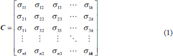
The diagonal elements of the matrix are the variances (.png/image(10)__60x19.png) ) and the off-diagonal are the covariances. Each variance contains information regarding the variation of only one measured item and the covariances contain information about the variation of two of the measured items. Now as the covariances represent the communal (or joint) variation; all non-communal variation is represented by the variances. Summing up all the elements of the matrix would give us the total variance present in the scale item Y, under the assumption of equal weights of the items (Nunnally, 1978).
) and the off-diagonal are the covariances. Each variance contains information regarding the variation of only one measured item and the covariances contain information about the variation of two of the measured items. Now as the covariances represent the communal (or joint) variation; all non-communal variation is represented by the variances. Summing up all the elements of the matrix would give us the total variance present in the scale item Y, under the assumption of equal weights of the items (Nunnally, 1978).
Alpha is defined as the proportion of the total variance that is attributable to a common source. Let .png/image(11)__20x23.png) denote the sum of all the elements of the matrix
denote the sum of all the elements of the matrix .png) and let
and let .png/image(13)__32x20.png) represent the sum of all the diagonal elements of matrix , then we can represent the ratio of non-communal variation to total variation as
represent the sum of all the diagonal elements of matrix , then we can represent the ratio of non-communal variation to total variation as

And we can express the ratio of communal variation to total variation as follows:
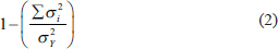
Table 1. The Four Measurement Models of CTT.
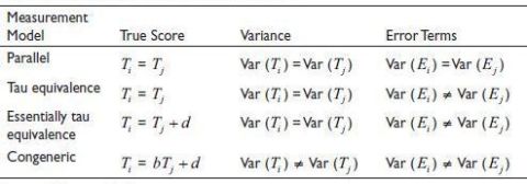
Source: Warrens (2016).
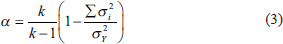
Equation (2) captures the essence of Cronbach’s alpha, however it suffers from a problem. Let us assume that a scale is made up of five perfectly correlated items. Then it should result in perfect reliability. In other words, Equation (2) should have the value of 1. But this would not be so as the correlation matrix will have a total of 25 entries, all equalling 1. The sum of the diagonals would be 5 and the sum of the matrix would be 25 and hence the value of Equation (2) would be .png/image(16)__125x20.png) . This happens because the total number of elements in the covariance matrix is
. This happens because the total number of elements in the covariance matrix is .png) and the number of elements on the diagonal are only
and the number of elements on the diagonal are only .png) leaving
leaving .png) off-diagonal elements. In Equation (2) the numerator is based on
off-diagonal elements. In Equation (2) the numerator is based on .png) values while the denominator is based on
values while the denominator is based on .png) values. To counteract for these differences in a number of terms, we multiply the formula by
values. To counteract for these differences in a number of terms, we multiply the formula by .png) or equivalently by
or equivalently by.png) thereby arriving at the formula for alpha:
thereby arriving at the formula for alpha:
If we assume that .png) is the average variance, then
is the average variance, then .png/image(25)__73x19.png) . Similarly,
. Similarly, .png) is the sum of all the elements in the matrix
is the sum of all the elements in the matrix .png) and if we assume that
and if we assume that .png) is the average covariance then
is the average covariance then .png/image(29)__144x23.png) . Substituting them in Equation (3) we get:
. Substituting them in Equation (3) we get:
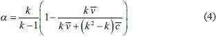
which on simplification gives:
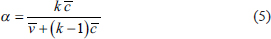
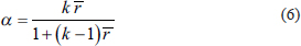
The formula in Equation (5) is based on unstandardised (raw) scores. To convert it to standardised scores, we need to recall that in a correlation matrix all the diagonal values equal 1; hence the average variance would also be one. The off-diagonal elements represent the correlations and hence the average covariance could be replaced by .png/image(30)__12x14.png) or the average intra-item correlation. This gives us the standardized alpha formula as
or the average intra-item correlation. This gives us the standardized alpha formula as
Issues with Cronbach’s Alpha
Despite its frequent use, Cronbach’s alpha has been criticised heavily by many researchers. One set of criticisms comes from the assumptions that are used to derive alpha (McNeish, 2017).
Issues Arising from Assumptions
Assumption of Tau-equivalence. One of the requirements for Cronbach’s alpha is the assumption of tau-equivalence which states that all the measurement items scale contribute equally to the construction of the scale. Any social researcher can easily see that such an assumption is impractical in the real world. Almost all the scales that are used in the real world are congeneric, meaning that the measured items contribute to the latent variable but with different importance (Raykov, 1997). Being a tau-equivalent measure means that alpha is not an exact measure of reliability but a lower bound provided that the errors are reasonably uncorrelated (Sijtsma, 2008).
Assumption of Normality and Continuous Items. One of the things to note in the derivation of alpha is that it is based on observed covariances and correlations between items. Statistical software estimates alpha using Pearson’s covariance matrix—which is known to be calculated on continuous data (Gadermann et al., 2012). On the other hand, the measurement items used to create the scales are usually interval or ordinal scales. This means that the covariance matrix so calculated would be biased downwards. This leads to lower alpha values because the relationships between the items would appear smaller than they are. The use of polychoric correlation is recommended for the calculation of alpha under such circumstances (McNeish, 2017). Another assumption is that of normality of the error terms and the true score. Cronbach’s alpha assumes that the error terms and the measurement items are normally distributed; but often empirical data shows non-normality and correlated errors. This means that Cronbach’s alpha does not reflect true reliability. Studies in the area have given mixed results—some arguing that Cronbach’s alpha is robust to deviations from non-normality (Zimmerman et al., 1993) while others argue it is susceptible to non-normality (Sheng & Sheng, 2012).
Assumption of Uncorrelated Error Terms. Another major requirement of the derivation of Cronbach’s alpha is that the error terms of the measurement items be uncorrelated to each other. Correlation of errors can arise due to several reasons like the order of measurement, respondent fatigue or the unforeseen multidimensionality of a scale. When errors are correlated, it is mostly found that they are correlated positively. This leads to an overestimation of Cronbach’s alpha (Gessaroli & Folske, 2002). While some of the errors can be minimised by randomising the test items, others are difficult to identify during the conceptualisation and data collection phase.
Assumption of Unidimensionality. Many researchers tend to believe that large alpha values indicate unidimensionality, or that the measurement items measure a single latent construct. But in real life, even pre-validated scales can show multidimensionality when used in a socio-economic context outside of the environment in which they were constructed. Multidimensionality comes to light when data is being analysed using factor analysis techniques and by that time it may be too late to reconstruct a new scale. Another confusion that occurs is that many researchers tend to believe that unidimensionality and internal consistency are the same—which is untrue. Internal consistency is defined as the interrelatedness of a set of items while unidimensionality is the degree to which items measure the same latent construct (Schmitt, 1996). Green et al. (1977) have pointed out that internal consistency is necessary but not sufficient for demonstrating unidimensionality. This means that large alpha values do not necessarily guarantee that the measurement items measure a single latent construct. It is possible that high values of alpha may be measuring the internal consistency of the construct and not unidimensionality.
Other Related Issues
Besides the above, there are other issues related to alpha. One of the most common beliefs is that alpha values greater than 0.70 provide excellent reliability. Cronbach (1951) never proposed any cut-off values for alpha. The value of .png/image(32)__54x11.png) seems to come from the work of Nunnally and Bernstein (1994). Over a period, this has become the standard benchmark over which all scale reliability is judged. In fact, many researchers have pointed out that there is no universal minimum acceptable reliability value for alpha. Any acceptable value depends on the type of application and what is being measured (Bonett & Wright, 2015).
seems to come from the work of Nunnally and Bernstein (1994). Over a period, this has become the standard benchmark over which all scale reliability is judged. In fact, many researchers have pointed out that there is no universal minimum acceptable reliability value for alpha. Any acceptable value depends on the type of application and what is being measured (Bonett & Wright, 2015).
Another issue that arises with alpha is that of the bounds. It can be seen from Equation (6) that when .png) , the value of
, the value of .png) and when
and when .png) the value of
the value of .png) . The extremely high value of alpha tends to indicate that the items on the scale are highly correlated. This could indicate issues of unidimensionality or problems of multicollinearity with scale items. As such it is recommended that alpha values >0.90 should be viewed with extreme caution. On the other hand, when
. The extremely high value of alpha tends to indicate that the items on the scale are highly correlated. This could indicate issues of unidimensionality or problems of multicollinearity with scale items. As such it is recommended that alpha values >0.90 should be viewed with extreme caution. On the other hand, when .png) the formula does not give a lower bound.
the formula does not give a lower bound.
In his original article Cronbach (1951) had demonstrated that alpha is the average of all possible split-half coefficients which could be calculated using the Spearman–Brown formula. This result positioned alpha as the expectation of split-half reliability values. This has led to the growing belief that alpha is a point estimate of reliability and as such it is sufficient to establish reliability. However, the reported value of alpha is the sample value (statistic) and contains sampling errors. Hence the reported value of alpha may not correctly reflect the reliability of the scale in question. It is always advisable to report a CI to give a better perspective to reliability (Bonett & Wright, 2015).
With so much criticism of alpha floating around it is surprising that it remains one of the most reported methods for reliability. In fact, many researchers conclude that the popularity of Cronbach’s alpha is due to inertia—reviewers and publishers look for alpha to give some sort of legitimacy to scale items. This was supported by the empirical work done by Hoekstra et al. (2019) in which they found that 74% researchers reported alpha because it was a common practice in the area while 53% reported it because the journal demanded it. In the same study, about 79% of the researchers mentioned that they consider 0.70 or more as a desirable level of alpha. Only about 20% of them suggested that the values be either a range of values or context-dependent.
Alternative to Alpha
Many alternatives to alpha have been proposed since then. It is not the intent to review all the alternatives; but a few of the most common ones are discussed here.
Alpha with CI
The problem with alpha is that researchers tend to report it as a point estimate. In statistics, a point estimate is considered the best guess estimate of the unknown population parameter. However, in the case of alpha, this is not the case as it clearly is a sample statistic and hence can be significantly biased. Interval estimation is a natural way of incorporating precision in statistical summary. One way of doing it is to use ‘bootstrapping’ using software like R and MATLAB. CI reporting is also present in SPSS and will be discussed in the seventh section. Dunn et al. (2014) have strongly recommended that alpha be always reported with the CI.
McDonald’s Omega
Another measure that has been regularly proposed is omega (McDonald, 1999). The .png) coefficient—which is congeneric in nature—uses the factorial analysis framework for estimating reliability and is expressed as
coefficient—which is congeneric in nature—uses the factorial analysis framework for estimating reliability and is expressed as
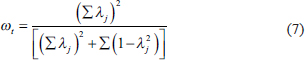
where .png/image(39)__14x19.png) is the loading of item
is the loading of item .png/image(40)__6x14.png) and
and .png) is the communality of the item . Now (1-)can be thought of as the uniqueness of the item and if we replace the same with
is the communality of the item . Now (1-)can be thought of as the uniqueness of the item and if we replace the same with .png) then the formula reduces to
then the formula reduces to
As the coefficient makes use of the factor loadings it tends to correct one of the key drawbacks of alpha—that is of unidimensionality. Under the condition of tau-equivalence, when the factor loadings are equal or extremely close to each other, it reduces to alpha. On the other hand, when the assumptions of tau-equivalence are violated then corrects the underestimation bias of alpha (Dunn et al., 2014). Various other studies have also found to be one of the the best alternatives for estimating reliability (Revelle & Zinbarg, 2008; Zinbarg et al., 2005; Zinbarg et al., 2006).
Another variant of omega was proposed by McDonald (1999) and is known as hierarchical omega (.png) ). It is used when errors in the measured items are correlated; or when there is more than one latent dimension present in the scale.
). It is used when errors in the measured items are correlated; or when there is more than one latent dimension present in the scale. .png) , calculates the contribution of each dimension to the total variance and corrects for the overestimation bias in multidimensional data. Under unidimensionality, and are identical. Most statistical software report under the assumption that scale is unidimensional.
, calculates the contribution of each dimension to the total variance and corrects for the overestimation bias in multidimensional data. Under unidimensionality, and are identical. Most statistical software report under the assumption that scale is unidimensional.
Greatest Lower Bound
The final measure that is discussed is known as the GLB (Woodhouse & Jackson, 1977). Under the assumptions of CTT and a single administration of the scale, the covariance matrix of observed scores (.png/image(45)__16x19.png) ) is decomposed into the sum of the covariance matrix of true scores (
) is decomposed into the sum of the covariance matrix of true scores (.png/image(46)__16x19.png) )and the error covariance matrix (
)and the error covariance matrix (.png/image(47)__16x18.png) ). The error covariance matrix () is diagonal with error variances on the main diagonal and off-diagonal are all zeros as per the assumptions of CTT. All three matrices are assumed to be positive semi-definite; that is, they have only positive eigenvalues. Then the GLB is defined as
). The error covariance matrix () is diagonal with error variances on the main diagonal and off-diagonal are all zeros as per the assumptions of CTT. All three matrices are assumed to be positive semi-definite; that is, they have only positive eigenvalues. Then the GLB is defined as
GLB represents the smallest possible reliability given the observed covariance matrix under the restriction that the sum of error variances is maximised. For a single-scale administration, true reliability is in the interval [GLB, 1]. However, if the scale administration can be repeated then GLB would provide a point estimate. The biggest problem in computing GLB is finding the trace of and various algorithms have been proposed for calculating the trace of . One of the most popular methods is that of GLB algebraic (.png/image(48)__40x22.png) ) (Moltner & Revelle, 2015). The algorithm is the most faithful to the original definition of GLB and has the added advantage of introducing a weight vector which weighs the items by their importance. Studies have demonstrated that tends to produce better results than alpha and omega (Wilcox et al., 2014).
) (Moltner & Revelle, 2015). The algorithm is the most faithful to the original definition of GLB and has the added advantage of introducing a weight vector which weighs the items by their importance. Studies have demonstrated that tends to produce better results than alpha and omega (Wilcox et al., 2014).
Finding the Alternatives
Given the drawbacks of Cronbach’s alpha and the availability of alternatives it is surprising that alpha is the most reported reliability coefficient. In many cases, researchers tend to report alpha values as generated by the software without giving much thought to the appropriateness of the scale. This is because they tend to use ‘standardized’ scales which they assume would be equally applicable in a context outside of the origin of the development of the scales (Maurya et al., 2023; Rao & Lakkol, 2023).
In this section, we demonstrate how to calculate the measures using SPSS and R statistical software. The data set used is ‘staffsurvey.sav’ (Pallant, 2016).1 The data set is a part of the staff survey held at Australian universities and has 10 questions on a five-point scale. These questions are scored on agreement and importance. In the SPSS data set q1a represents the score of statement 1 on agreement and q1im represents the score on importance. The analysis is done on the agreement responses only.
Using SPSS to Generate CI for Alpha
To generate the CI for alpha we need to use the menu sequence .png/image(50)__304x17.png) . This opens the RELIABILITY ANALYSIS dialogue box. On the bottom right we have the Model drop-down selector which allows us to select Alpha, Split-Half, Gutmann (all lambda’s), parallel and strict-parallel modes. On the top right is the statistics button. Clicking on this button brings up the RELIABILITY ANALYSIS: STATISTICS dialog box. Next, we need to click on the Intraclass Correlation Coefficient and select the CI. Figure 1 shows the steps in detail. Now we click on continue and finally on the OK button to run the analysis. The output from SPSS is shown in Table 2.
. This opens the RELIABILITY ANALYSIS dialogue box. On the bottom right we have the Model drop-down selector which allows us to select Alpha, Split-Half, Gutmann (all lambda’s), parallel and strict-parallel modes. On the top right is the statistics button. Clicking on this button brings up the RELIABILITY ANALYSIS: STATISTICS dialog box. Next, we need to click on the Intraclass Correlation Coefficient and select the CI. Figure 1 shows the steps in detail. Now we click on continue and finally on the OK button to run the analysis. The output from SPSS is shown in Table 2.
The single measure intraclass correlation is the average intra-item correlation and the average measure intraclass correlation is the alpha value along with the 95% CI. The 95% CI has the value of [0.824, 0.865] which suggests that these set of items provides excellent reliability.
Using R and the psych Package
In the R ecosystem, the package psych (Revelle, 2023) provides a useful addition to the repertoire for the calculation of various reliability measures. The same data set was analysed using the psych package and the results are presented below. The code is provided in Annexure A.
Figure 1. How to Calculate Alpha Confidence Intervals in SPSS.

Source: The snapshot is taken by the author in IBM SPSS Statistics version 21.
Table 2. Intraclass Correlation Coefficient Table as Generated by SPSS.
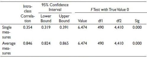
Source: Computed from the staffsurvey.sav data set by the author.
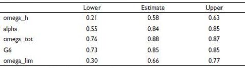
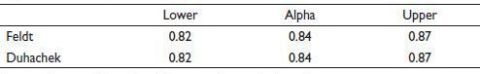
The alpha() command reports raw alpha, standardised alpha, Guttman’s .png) , the average value of intraclass correlations and other statistics. It also provides the 95% CI of alpha using the older Feldt et al. (1987) and the newer Iacobucci and Duhachek (2003) methodology.
, the average value of intraclass correlations and other statistics. It also provides the 95% CI of alpha using the older Feldt et al. (1987) and the newer Iacobucci and Duhachek (2003) methodology.
Based on the output of alpha it may be concluded that the items used in the scale are extremely reliable. However, when we run the omega() command the software reports ‘omega total ’ and omega hierarchical along with a bunch of other statistics. As omega is based on a factor analysis framework it also produces a graph showing an estimated number of factors along with the interrelations between the various scale items. Table 3 provides the output of the omega command.
The output shows the alpha value, Guttman’s and the omega hierarchical, omega hierarchical asymptotic and omega total values. Table 3 provides a completely different take on the outputs of Table 4—as the values are calculated using multiple random splits. The lower bound of alpha is 0.55 which automatically makes the scale a suspect even though the upper bound and the estimated values are consistent with Table 4. The omega_tot values seem excellent; but the omega_h and omega_lim values are extremely problematic.
Table 3. Output for the Omega Command.
Source: Computed from the staffsurvey.sav data set by the author.
Table 4. 95% Confidence Boundaries of Alpha.
Source: Computed from the staffsurvey.sav data set by the author.
Scale development in social sciences is majorly based on the assumption that the items in the scale measure a single latent variable. However, the internal structure of the scale is not taken into consideration. Omega uses the Schmid–Leiman transformation to identify the unidimensionality of the scale (Schmid & Leiman, 1957). Figure 2 shows the graphical output for the scale items.
The pictorial output of omega shows that there is a ‘third order factor’ denoted by g and there are three second order factors namely F1, F2 and F3. Another interesting thing to note is that g relies on eight measured variables. F2 seems not to be correlated with any of the measured variables while the bulk of measured variables load on F1. Item q8a loads negatively on F1 and either is a reversed measurement (in which case it needs to be corrected) or it is not a part of the measurement indicating that it may be needed to be dropped from the analysis. Thus, the omega analysis provides a deeper insight into the scale development process. Readers attempting to replicate the analysis should note that as the splits are random (n.iter = 10) they may get slightly different figures.
calculation requires the covariance matrix and the covariance matrix can be used in the glb.algebriac() command to get the values. The function does not check for positive semi-definiteness of the covariance matrix. In case of empirical matrices with small sample sizes, calculated values of may be strongly biased upwards. Table 5 provides the output of GLB.
GLB represents the smallest possible reliability given the observed covariance matrix under the restriction that the sum of error variances is maximised. For a single-scale administration, true reliability is in the interval [GLB, 1]. Variable q4a, q5a and q9a may seem problematic as their estimates are greater than 1. Similarly, q1a and q8a can also be a cause of concern due to their low estimates.
Figure 2. The Omega Factor Analysis Output (sl = TRUE).
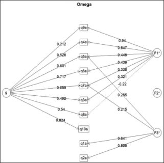
Source: Computed from the staffsurvey.sav data set by the author.
Table 5. Output of the glb.algebraic() Command.
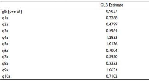
Source: Computed from the staffsurvey.sav data set by the author.
In this section, we have calculated alpha, omega and GLB. Based on alpha we may have concluded that the scale is a robust scale but analysis with omega and GLB tends to indicate issues with the items and consequently the scale development process.
Summary
This article does not criticise Cronbach’s alpha or claim to encompass all reliability calculations and reporting methods. The reliability literature is broad and over a century old. Due to the widespread use of alpha in social science and the lack of understanding surrounding it, this article aims to educate researchers about the various problems and associated issues with alpha and provide them with easy-to-calculate alternatives that provide deeper insights into reliability. It is suggested that researchers should use two or more different metrics to better comprehend the reliability of scales. With the passage of time, it has become necessary to use and report better measures of reliability social science literature.
Annexure A: Code for Analysis
## Install the necessary packages.
install.packages("psych", dependencies = TRUE)
install.packages("psychTools", dependencies = TRUE)
install.packages("foreign", dependencies = TRUE)
install.packages("tidyr", dependencies = TRUE)
## Load the packages and make it available to R
library(psych)
library(psychTools)
library(foreign)
library(tidyr)
## Read in the SPSS File using a dialog box.
spssdb <- file.choose()
myData <- read.spss(spssdb, use.value.labels = FALSE, to.data.frame = TRUE,
use.missings = FALSE)
## See whether the data set was read in correctly. The dim() command should give
## the output as 536 30 indicating 536 rows and 30 columns
head(myData)
dim(myData)
## Drop all rows with NA or missing values
myData2 <- myData %>%
drop_na()
## myData2 should have 330 rows and 30 variables
dim(myData2)
## Copy all the column variables which have “agreement scores” to a new dataframe
## The new dataframe should have 330 rows and 10 columns
newDf <-myData2[, c(6, 8, 10, 12, 14, 16, 18, 20, 22, 24)]
dim(newDf)
## Calculate Alpha
alpha(newDf, use = "complete", impute = "mean", check.keys = TRUE)
print(alpha.ci(.84, 330, p.val=.05, n.var = 10))
## Calculate Omega
omega(newDf, n.iter = 10, digits = 4, sl = TRUE)
## Convert the dataframe to a covariance matrix and calculate the GLB
covMatrix <- cov(newDf)
glb.algebraic(covMatrix)
Acknowledgement
The author is grateful to the anonymous referees of the journal for their extremely useful suggestions to improve the quality of the article. Usual disclaimers apply.
Declaration of Conflicting Intere
The author declared no potential conflicts of interest with respect to the research, authorship and/or publication of this article.
Funding
The author received no financial support for the research, authorship and/or publication of this article.
Note
ORCID iD
Rohit Vishal Kumar https://orcid.org/0000-0001-5594-0129
Bonett, D. G., & Wright, T. A. (2015). Cronbach’s alpha reliability: Interval estimation, hypothesis testing, and sample size planning. Journal of Organizational Behavior, 36(1), 3–15.
Brown, W. (1910). Some experimental results in the correlation of mental abilities. British Journal of Psychology, 3, 296–322.
Cronbach, L. J. (1947). Test 'reliability': Its meaning and determination. Psychometrika, 12, 1–16.
Cronbach, L. J. (1951). Coefficient alpha and the internal structure of tests. Psychometrika, 16(3), 297–334.
Cronbach, L. J., & Shavelson, R. J. (2004). My current thoughts on coefficient alpha and successor procedures. Educational and Psychological Measurement, 64(3), 391–418.
DeVillis, R. F. (2003). Scale development: Theory and applications. Sage Publications.
Dunn, T. J., Baguley, T., & Brunsden, V. (2014). From alpha to omega: A practical solution to the pervasive problem of internal consistency estimation. The British Journal of Psychology, 105, 399–412.
Feldt, L. S., Woodruff, D. J., & Salih, F. A. (1987). Statistical inference for coefficient alpha. Applied Psychological Measurement, 11, 93–103.
Gadermann, A. M., Guhnand, M., & Zumbo, B. D. (2012). Estimating ordinal reliability for Likert-type and ordinal item response data: A conceptual, empirical, and practical guide. Practical Assessment, Research & Evaluation, 17, 1–13.
Gessaroli, M. E., & Folske, J. C. (2002). Generalizing the reliability of tests comprised of testlets. International Journal of Testing, 2, 277–295.
Goodenough, F. L. (1936). A critical| note on the use of the term “reliability” in mental measurement. Journal of Educational Psychology, 27, 173–178.
Green, S. B., Lissitz, R. W., & Mulaik, S. A. (1977). Limitations of coefficient alpha as an index of test unidimensionality. Educational and Psychological Measurement, 37, 827–838.
Hoekstra, R., Vugteveen, J., Warrens, M. J., & Kruyen, P. M. (2019). An empirical analysis of alleged misunderstandings of coefficient alpha. International Journal of Social Research Methodology, 22(4), 351–364.
Iacobucci, D., & Duhachek, A. (2003). Advancing alpha: Measuring reliability with confidence. Journal of Consumer Psychology, 13(4), 478–487.
Kuder, G. F., & Richardson, M. W. (1937). The theory of the estimation of test reliability. Psychometrika, 2, 151–160.
Maurya, A. M., Padval, B., Kumar, M., & Pant, A. (2023). To study and explore the adoption of green logistic practices and performance in manufacturing industries in India. IMIB Journal of Innovation and Management, 1(2), 207–232. https://doi.org/10.1177/ijim.221148882
McDonald, R. (1999). Test theory: A unified treatment. Lawrence Erlbaum Associates.
McNeish, D. (2017). Thanks coefficient alpha, we’ll take it from here. Psychological Methods, 23(3), 412–433.
Moltner, A., & Revelle, W. (2015). Find the greatest lower bound to reliability. Web Article.
Novick, M. R. (1966). The axioms and principal results of classical test theory. Journal of Mathematical Psychology, 3, 1–18.
Nunnally, J. C. (1978). Psychometric theory (2nd ed.). McGraw-Hill.
Nunnally, J. C., & Bernstein, I. H. (1994). The assessment of reliability. Psychometric Theory, 3, 248–292.
Pallant, J. (2016). SPSS survival manual: A step by step guide to data analysis using IBM SPSS (6th ed.). Open University Press.
Rao, A. S., & Lakkol, S. G. (2023). Influence of personality type on investment preference and perceived success as an investor. IMIB Journal of Innovation and Management, 1(2), 147–166. https://doi.org/10.1177/ijim.221148865
Raykov, T. (1997). Estimation of composite reliability for congeneric measures. Applied Psychological Measurement, 21, 173–184.
Revelle, W. (2023). psych: Procedures for psychological, psychometric, and personality research. Northwestern University. https://CRAN.R-project.org/package=psych
Revelle, W., & Zinbarg, R. E. (2008). Coefficients alpha, beta, omega, and the glb: Comments on Sijtsma. Psychometrika, 74(1), 145–154.
Schmid, J., & Leiman, J. (1957). The development of hierarchical factor solutions. Psychometrika, 22(1), 53–61.
Schmitt, N. (1996). Uses and abuses of coefficient alpha. Psychological Assessment, 8, 350–353.
Sheng, Y., & Sheng, Z. (2012). Is coefficient alpha robust to non-normal data? Frontiers in Psychology, 3, 34.
Sijtsma, K. (2008). On the use, the misuse, and the very limited usefulness of Cronbach’s alpha. Psychometrika, 74(1), 107–120. https://www.ncbi.nlm.nih.gov/pmc/articles/PMC2792363/pdf/11336_2008_Article_9101.pdf
Spearman, C. (1910). Correlation calculated with faulty data. British Journal of Psychology, 3, 271–295.
Warrens, M. J. (2016). A comparison of reliability coefficients for psychometric tests that consist of two parts. Advances in Data Analysis and Classification, 10, 71–84. https://doi.org/10.1007/s11634-015-0198-6
Wilcox, S., Schoffman, D. E., Dowda, M., & Sharpe, P. A. (2014). Psychometric properties of the 8-item English arthritis self-efficacy scale in a diverse sample. Arthritis, 2014, 1–8.
Woodhouse, B., & Jackson, P. H. (1977). Lower bounds for the reliability of the total score on a test composed of non-homogeneous items: II: A search procedure to locate the greatest lower bound. Psychometrika, 42(4), 579–591.
Zimmerman, D. W., Zumbo, B. D., & Lalonde, C. (1993). Coefficient alpha as an estimate of test reliability under violation of two assumptions. Educational and Psychological Measurement, 53, 33–49.
Zinbarg, R. E., Revelle, W., Yovel, I., & Li, W. (2005). Cronbach’s alpha, Revelle’s beta, and McDonald’s omega: Their relations with each other and two alternative conceptualizations of reliability. Psychometrika, 70(1), 123–133.
Zinbarg, R. E., Yovel, I., Revelle, W., & McDonald, R. P. (2006). Estimating generalizability to a latent variable common to all of a scale’s indicators: A comparison of estimators for omega. Applied Psychological Measurement, 30(2), 121–144.
