Introduction

In order to achieve India’s vision of a five-trillion economy in the next five years, a safe, reliable and robust financial sector is crucial. Banking structures, including the country’s central bank, play a very important role in expanding and widening the financial system, fostering savings institutionalisation and investment and pushing the country’s economic growth (Bapat, 2012; Ghosh & Saggar, 1998; Velayudham, 1989). Currently banking system in India is responsible for regulating and managing over 70% of the funds that flow through financial sector in the country. The fluctuations in banking industry affect the economic growth of a country negatively (Moshirian & Wu, 2012). Non-performing assets (NPAs) are one of the key and most formidable glitches that have traumatised the whole banking sector in developing countries long afore economic liberalisation in 1991 (Ghosh & Saggar, 1998). An NPA is demarcated as default of payment for interest and/or instalment of principal for a credit facility for a specified period of time (Khan, 2007). Many researchers have investigated the relationship between loan growth and NPAs that concluded that when banks follow aggressive loan growth (though favourable for its business), these loans may turn into NPAs in future (Clair et al., 1992; Keeton et al., 1999). Several studies show the influence of NAPs on bank’s effectiveness and overall productivity (Bawa et al., 2019; Sharma et al., 2020).

The functioning, profitability and performance of a banking system in the country are largely dependent on the amount of NPAs of the banks operational in the country. The effectiveness of the bank can be measured using a range of bank ratios, such as operating ratios, profitability ratios and liquidity ratios (Halkos & Salamouris, 2004; Kumbirai & Webb, 2010; Yeh, 1996). The financial enactment of a bank is usually judged by net profit ratio (NPR), return on assets (ROA), return on equity (ROE) and net interest margin, liquidity risk is calculated by the liquidity ratio, and capital adequacy ratio presents the idea of solvency position of the bank. A very high gross NPA (GNPA) ratio specifies the poor quality of the bank’s asset while high net NPA (NNPA) is an indicator of overall health of the bank. In the loan portfolio, NPAs impact operating performance, which in turn disturbs the profitability, liquidity and solvency of cooperative bank (Michael, 2006; Purbaningsih & Fatimah, 2014). Different studies indicate that credit risk has a major adverse bearing on profitability and liquidity (Ruziqa, 2013). The studies discuss the positive association between the liquidity of banks and the adequacy of capital, the portion of non-performing loans and interest rates on loans and interbank transactions (Vodova, 2011).

In the light of above discussion, we apply the panel regression model on current 30 banks both from public and private sectors to measure the impact of the GNPA ratio (intended as GNPAs as a percentage of advances) on profitability, liquidity and solvency ratios. NPA has insignificant inverse relationship with net profit of the bank. The existence of NPAs has an important impression on the earning capacity and profitability of banks. An elevated amount of NPAs specifies a bulky number of credit evasions, which affects bank profitability and net worth (Dudhe, 2017). Several studies also indicate that the increase in NPA negatively affects the ROA and ROE of banks. The increase in NPAs is responsible for increase in operating costs leading to decrease in cash flow from operating activities and because of this the cash flow margin ratio also goes down. Banks performance largely depends on available liquidity. Higher NPA not only impacts the liquidity of banks, but also force the banks to have higher investment in liquid assets. It also forces the banks to borrow money or raise short-term deposits. The operating cash flow ratio indicates the banks’ capacity to discharge the current liabilities form the cash generated from operation. But the operating cash flow is inversely impacted by increased NPA level. In banks’ books, loans and advances are primary items of assets, which have the loss potential due to loan defaults (NPA). The capital adequacy ratio (CAR) is the ratio of total capital of bank to risk weightage assets and directly related to quality of assets (loans and advances). NPA has an inverse relation with CAR. Keeping all the above-mentioned points in mind, the current topic has been taken to examine the impact of NPAs on Indian banking structure.

The research article goes in a subsequent way: The following segment provides a particularised overview of relevant researches and empirical literature in this field, followed by the study’s purposes and justification. In the following sections, the methodology and methodological approach, as well as the data used, are explained, followed by data exploration and the calculation of empirical results. The final piece describes the discoveries, draws an inference and summarises the article, highlighting the study’s major offerings to the literature.

Review of Related Literature

In this section, we present a wide survey of existing literature related to the offered topic. In their study, Seenaiah et al. (2015) conclude that operating profits, wage bills, NPAs and net interest margin affect the profitability of the Indian banks, whereas the priority sector advancing does not have any influence on the bank’s productivity in India. It is further stated that the banks should reduce its operational expenses so that the net interest margin can increase, as presently it is affecting the banks’ profitability in India. Jaisinghani and Tandon (2015) have tried to foresee the NPAs of the Indian banks by using logit and probit models. Barua et al. (2016) in their study stated that profitability is affected by the market concentration and the bank-specific macro variables. The study further concludes that the leverage, capitalisation credit risk and ownership structure are the important factors of the Indian bank’s productivity. The study further states that the pecuniary crunch had no bearing on the profitability of the Indian banks. Mostak Ahamed (2017) has found that the non-interest income activities progress the profitability of the Indian banks and in particular to those which have a lower asset quality. The author concludes that the diversification activities increase the profitability in particular of those banks that have a low-quality asset. Vidyarthi et al. (2017) have concluded that the public sector banks need more attention with respect to NPAs management as it is affecting the profitability and efficiency exponentially. Singh and Sharma (2018) in their study formed the opinion that capital adequacy ratio, deposits and profitability influence Indian bank liquidity absolutely, whereas bank size, NPAs and net interest margin disturb Indian banks’ liquidity negatively. Goyal and Verma (2018) in their learning found the determinants of credit and NPAs. Their findings support the notion that past credit, higher interest rates and low growth have contributed to an increase in NPAs. However, the other determinants such as control and ownership structure have no noteworthy influence on the NPAs. Whereas in the study conducted by Bawa et al. (2019), authors have concluded that the liquidity of the Indian banks is not considered as a significant factor because the Reserve Bank of India as per its standard policy monitors the liquidity of the Indian banks on weekly basis and this protects the banks from the liquidity crisis. Swami et al. (2019) in their finding list the poor operating efficiency, lower capital base and reducing profits as the key factors in reducing the asset quality of the banks. Ramesh (2019) in his study found that ROE, loan maturity and credit-to-deposit ratio have an adverse connection with the NNPAs, whereas the operating expense and capital adequacy ratio have an inconsequential affiliation with the NNPAs. In addition, the author has stated that priority sector loans, non-interest income and collateral values have all played a significant role in increasing NPAs in public sector banks. Gaur and Mohapatra (2020) in their study explored the NPA–profitability relationship in the Indian banking sector. In their study, they have used panel data set of 37 scheduled commercial banks for the period of 14 years. They have concluded that due to the presence of heteroscedasticity, a high standard error is recorded which leads to a high adverse correlation between NPA and two profitability procedures, that is, ROA and ROE. Gupta and Kashiramka (2020) in their study analyse the importance of liquidity formation for instituting the financial stability of the banks. The authors conclude that the liquidity creation increases the financial stability of the banks as per its size. Further, they conclude that the private sector banks are more financially stable than the government sector banks. However, Thomas and Singh (2020) in their study found that the upsurge in the NPA ratio does not theoretically increase riskier advancing. They support the notion ‘too-big-to fail’ through the evidence stating that the big banks must have some incentives that is why they are taking higher risk and have high NPA ratios. Mehta and Kaushik (2020) have stated that the capital blocked or lost in NPA in various banks has a straight impact on the bank’s profitability, liquidity and its market value. Further, they conclude in their study that the increase in NPA has an adverse relationship with earning per share (EPS) and market per share (MPS).

From the conclusive summary of related literature, a gap can be seen for study on the offered topic in context of the Indian banking system. Most of the researchers discuss the determinants of NPAs, bank specifics, internal and external factors and macro-economic variables causing NPAs. The effect of NPAs on the operating performance and profitability of commercial banks in the country is also being studied in several studies but it is limited to certain ratios. So, the current study has been undertaken to test the impact of the GNPA ratio on profitability, liquidity and solvency in context of Indian banks.

Methodology: Data, Sample Frame and Empirical Model

In the current study, we have used the panel data of 30 banks (12 government sector and 18 private sector banks) from 2014 to 2020 (7 years). The data have been sourced from Prowess (CMIE) and www.moneycontrol.com. The description of variables taken for current study is as follows.

The Variables

The variables considered initially to develop the empirical model are defined below.

GNPAR: Gross Non-performing Assets Ratio (GNPA as percentage of advances)
NPR: Net Profit Ratio (Net Profit after Tax/Income from Financial Services + Interest Income)
ROA: Return on Assets (Net Profit/Average Total Assets)
ROE: Return on Equity (Net Profit/Shareholder’s Equity), Shareholder’s Equity = Equity Capital + Reserves and Surplus
CFMR: Cash Flow Margin Ratio (Cash Flow from Operating Activities/Total Revenue)
Here, Total Revenue = Income from Financial Services + Interest Income
CTR: Current Ratio (Current Assets/Current Liabilities)
ATR: Acid Test Ratio (Quick Assets/Quick Liabilities), Quick Assets = Current Assets (as inventories are 0) And Quick Liabilities = Current Liabilities–Short Term Borrowings, Loans, O/D
CR: Cash Ratio (Cash and Cash Equivalents/Current Liabilities)
OCFR: Operating Cash flow Ratio (Cash from Operating Activities/Current Liabilities)
CAR: Capital Adequacy ratio{(Tier 1 capital + Tier 2 capital)/Risk Weighted Assets}

Econometric Modelling of Panel Regression Models: Includes the Following Steps

First, we consider the model identification and then diagnostic testing of the models. There are certain assumptions for applying panel data regression. Assumptions about the properties of initial conditions play an important role in the identification of a suitable model. There subsists a set of essential and adequate documentation settings for panel models. The preceding set of the panel equation showing usual fixed effect is as follows:

where Y_it shows the vector of the dependent variable, X_it is the vector of an observable regressor, β is the unknown coefficient, α_i is the individual effect, ξ_t is the time effect and ε_it shows the vector of error term.

Pre-testing for stationarity in short-panel data models is a matter of interest (not necessary for short panel data). In the current study, we have used Levin–Lin–Chu test for checking the presence of unit root in the panel data.

If individual effect u_i (cross-sectional or time-specific effect) does not exist (u_i = 0), ordinary least squares (OLS) produces competent and steady parameter estimates. So, the first requirement (for model identification) is to check whether all Coefficients are Continuous across Time and Individuals. Pesaran CD test has been used to check individuality of each cross-sectional unit. In the literature, the model based on time invariant but individuality in cross-sectional unit is known as the fixed effects (regression) model (FEM). Next, we check time effect with the help of Wald joint test on time dummies. The general preservative properties α_i + ξ_t being an unusual case of multiple interactive properties seems to be less observed. But once indicated, it converts insignificant and apparent (Bai, 2009). These additive properties can be detached by the within group renovation (least-squares dummy variables).

The next step in the identification process is to check exogeneity which indicates that the expected value of error terms should be zero (necessary to apply OLS). Then we check autocorrelation between the error term and regressor. Durbin–Watson test statistic has been used to check auto-correlation. Next, we check homoscedasticity in the error term. The homoscedasticity has been checked with Breusch–Pagan test. Ahn et al. (2001) reflect the condition of fixed T and noted that the least-squares method fails to present reliable estimator if serial correlation or heteroscedasticity is extant in ε_it. In this condition, dynamic panel regression models are more suitable.

To compare a random effect model to its fixed complement, the Hausman (1978) specification test was used. If the null hypothesis of uncorrelated individual effects with other regressors is not rejected, a random effect model is found to be more suitable than a fixed effect model.

Then next step is to do the diagnostic checking of models applied. The diagnostic testing involves whether intercept and regressors do not disrupt any Gauss–Markov assumption; a fixed effect model is still BLUE. For diagnostic checking of models, we test following assumptions. First assumption is to check whether the mean value of the error term is zero. Second, homoscedasticity has been tested by applying Breusch–Pagan test. The third assumption is checking endogeneity which means whether error terms are correlated with independent variables. Then auto-correlation has been checked using Durbin–Watson test. If the Durbin–Watson test reading is less than 1, it shows negative auto-correlation and if it is more than 3, it shows positive auto-correlation. The value of test between 1 and 3 shows no auto-correlation.

Analysis

Empirical Results

Table 1 demonstrates the summary statistics of independent and dependent variables taken for the current study where GNPAR is the regressor and NPR, ROA, ROE, CFMR, CTR, ATR, CR, OCFR and CAR are dependent variables.

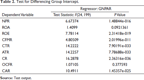
Table 2 demonstrates the results of test conducted to check the common group intercept. The results show that the data are not poolable (rejects the hypothesis that the groups have common intercept) in case of NPR, ROE, CFMR, CTR, ATR, CR and CAR for both the regressors, that is, GNPAR so pooled model is not suitable for current data set. If the entire groups are found to have common intercept, OLS produces efficient and consistent parameter estimates. In case of variables ROA and OCFR, the null hypothesis of group having a common intercept is accepted (so OLS can be applied).

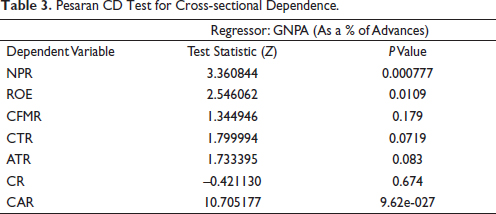
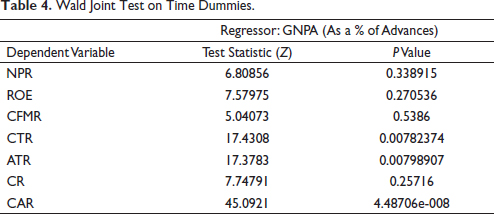
Table 3 and Table 4 present the cross-sectional dependence or individual effect and time effect, respectively. The Pesaran CD test for cross-sectional independence has the null hypothesis that there is no cross-sectional or individual effect. We have not calculated cross-sectional and time effect in case of variables ROA and OCFR as OLS will be applied to regress these variables. The independent variable GNPAR shows individual effect only in case of NPR, ROE and CAR. There is no individual effect in variables CFMR, CTR, ATR and CR.

The time effect has been tested using Wald Joint test. The test has the null hypothesis that there is no time effect. On the basis of results of Table 4, only variables CTR, ATR and CAR have time effect other variables do not have time effect. In conclusion we can say that the fixed/random effect model will be applied.

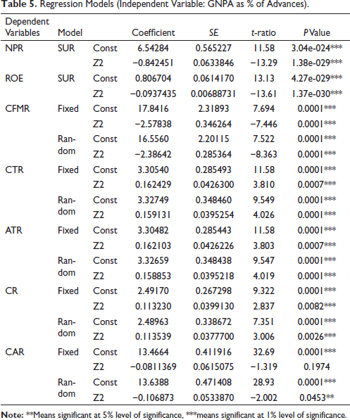
Table 5 reveals the results of the regression model. The variables NPR and ROE have only individual effect but no time effect so seemingly unrelated regression (SUR) models have been used. For other variables, we have used fixed and random effect models. The outcomes of SUR models show that GNPAR significantly impacts NPR and ROE ratio at 1% level of significance. Both NPR and ROE share inverse association which shows both NPR and ROE are negatively impacted by GNPAR. We can also conclude the impact of GNPAR on CTR, ATR and CR (at 1% level of significance) and CAR (5% level of significance). CFMR (return on equity) and CAR (capital adequacy ratio) are seen to have negatively impacted by GNPAR.

Table 6 displays the result of rho, joint and Hausman tests. Rho is the variance in dependent variable due to individual effect or individual specific term. From the results of Table 6, we see very less individual impact on dependent variables due to individuality of banks. Hausman test is used to compare the better fit between fixed effect and random effect models. Hausman test has the null hypothesis that GLS estimates are consistent. On acceptance of the hypothesis, we can take the random effect model as a better fit model. It can be seen from results that in case of all the variables (except CAR), the null hypothesis that GLS estimates are consistent has been accepted so the random effect model is more suitable. In case of CAR, the fixed effect model is more suitable.

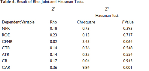
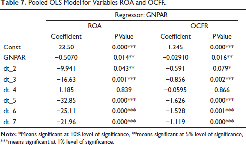
Table 7 put forth the results of OLS models (run for variables ROA and OCFR) which include time dummies as well. We see that GNPAR has a significant impact on both ROA and OCFR (at 5% level of significance). The time dummies of both the variables are also significant (at 1% level of significance) for all the years except 2017.

Diagnostic Checking

In this section, we examined whether the intercept and regressors violate any Gauss–Markov assumption; a fixed effect model remains BLUE. The results of diagnostic checking have been reported in Table 8. First assumption in this direction is to check whether mean value of error term is zero (to check this mean value of disturbance has been calculated). As per the results, it can be said that mean is almost zero in all the panel series (Column: Assumption 1). Then homoscedasticity has been checked using Breusch–Pagan test. As per the result that null hypothesis that there is homoscedasticity has been rejected (except variables ROA and OCFR). To control this problem of heteroscedasticity we have applied robust standard error. Next, we check the endogeneity that is to check whether error terms are correlated with independent variables. The correlation between the error term and independent variable is also close to zero in all variables so the endogeneity is not reported. So, the data are free from the problem of endogeneity. Then auto-correlation has been checked using Durbin–Watson test. If the Durbin–Watson test reading is less than 1, it shows negative auto-correlation and if it is more than 3 it shows positive autocorrelation. The value of test between1 to 3 shows no auto-correlation. As per the results of Durbin–Watson test all the variables are free from auto-correlation. So, we can say that the model developed for the study is fit as it clears all Gauss–Markov assumptions.

Discussion and Conclusions

For any bank, loans and advances are integral part of operation, but at the same time it is like a double-edged sword, if the quality of assets is non-performing in nature. It not only leads to non-recovery of loans but also stops the credit creation process subsequently. Beside these, NPA lowers the margins of banks and force the banks for higher provisions. The empirical outcomes offered in the current research ranges data from 2014 to 2020. The study replicates the findings of Louzis et al. (2012) in terms of bank size and NPA ratios; the larger the bank, the higher the NPA ratio. As per the findings of current study we can conclude that NPR is significantly impacted by NPA and inverse association indicates the fall in NPR with increasing NPAs. Further we found that cash flow margin ratio is impacted by GNPA ratio, negatively. So, we can conclude the negative association of cash flow margin with NPAs depending on the quantum of NPAs as a proportion to its advances. The ROA ratio is impacted by NPAs sharing negative association with it which implies the decrease in the ROA ratio with increasing NPAs. ROE is impacted by NPAs negatively. The current ratio and acid test ratio also have significant impact on GNPAs ratio. Cash ratio is also impacted by GNPAs ratio. Here also it can be concluded that cash ratio is impacted by GNPAs depending on their proportion in context of advances. The operating cash flow is also negatively impacted by NPAs. The capital adequacy is also seen to be impacted by GNPA ratio negatively. So, it can be said that the percentage portion of NPAs with advances specifies the connection between capital adequacy ratio and NPAs which is an inverse association amid the two.

The proposed study also guides to study the impact on NPAs on some more ratios related to operating efficiency and profitability of banks. Current study is limited to the Indian banking system so there is an ample scope for testing the same in global context taking a bigger and broad panel data.

Economic Implication

The study can provide valuable guidelines for policymakers to frame policies in the Indian banking system as a part of banking reform committees. These policies can be beneficial for the bankers, depositors, investors and the management to assess how the GNPA affects the profitability, liquidity and solvency of the banks. Further, they can also establish an affiliation between the capital adequacy and the NPAs.

Acknowledgement

The researchers are grateful to the journal’s unspecified referees for their really helpful recommendations to improve the article’s quality. The standard disclaimers apply.

Declaration of Conflicting Interests

The authors declared no potential conflicts of interest with respect to the research, authorship and/or publication of this article.

Funding

The authors received no financial support for the research, authorship and/or publication of this article.